Subplots in Matplotlib
Subplots in Matplotlib allow you to create multiple plots within the same figure, making it easy to compare different datasets or visualize related information side by side.
Creating Subplots
To create subplots, you use the subplots() function, which returns a figure object and an array of axes objects. Each axis represents a separate plot within the figure.
# Creating a 2x2 grid of subplots
fig, axs = plt.subplots(2, 2)
With just one line of code, you’ve created a 2×2 grid of subplots.
Now let’s create a simple example of subplots. Imagine you have two sets of data, and you want to compare their trends side by side.
Example:
import matplotlib.pyplot as plt
import numpy as np

# Generating some sample data
x = np.linspace(0, 10, 100)
y1 = np.sin(x)
y2 = np.cos(x)

# Creating a 1x2 grid of subplots
fig, axs = plt.subplots(1, 2, figsize=(10, 4))  # figsize adjusts the size of the entire canvas

# Plotting on the first subplot
axs[0].plot(x, y1, color='blue')
axs[0].set_title('Sine Function')

# Plotting on the second subplot
axs[1].plot(x, y2, color='green')
axs[1].set_title('Cosine Function')

# Adding labels to the entire figure
fig.suptitle('Comparing Sine and Cosine Functions')

# Displaying the plots
plt.show()
In this example:
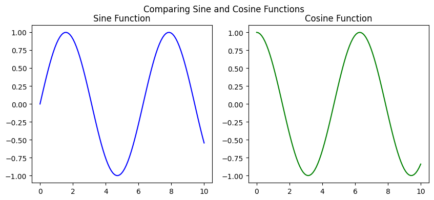
- We generate sample data using NumPy for the x-axis and two different y-axes (sine and cosine functions).
- We create a 1×2 grid of subplots using
plt.subplots(1, 2), indicating one row and two columns. - We access each subplot using the
axsarray and plot the corresponding data. - Titles are added to each subplot, and an overall title is added to the entire figure.
Now you have a beautifully organized canvas comparing the trends of the sine and cosine functions side by side.
Output:
Different Plots on Subplots
Let’s create a scenario where we have data representing the growth of plants under different conditions. We’ll use line plots, scatter plots, bar plots, and histograms to showcase various aspects of the data on individual subplots.
We start by importing the necessary libraries (matplotlib.pyplot and numpy) and generating sample data representing the growth of plants under three different conditions over a span of five days.
import matplotlib.pyplot as plt
import numpy as np

# Generating sample data
days = np.array([1, 2, 3, 4, 5])
condition1 = np.array([2, 5, 8, 11, 14])
condition2 = np.array([1, 3, 7, 9, 13])
condition3 = np.array([3, 6, 9, 12, 15])
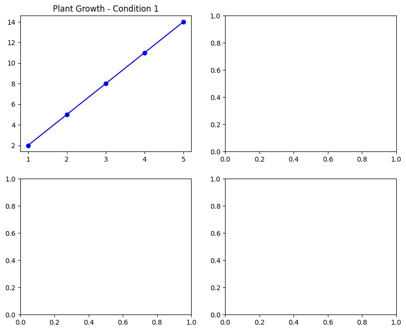
This line sets up a 2×2 grid for subplots within a figure and defines the figure size.
# Creating a 2x2 grid of subplots
fig, axs = plt.subplots(2, 2, figsize=(10, 8))
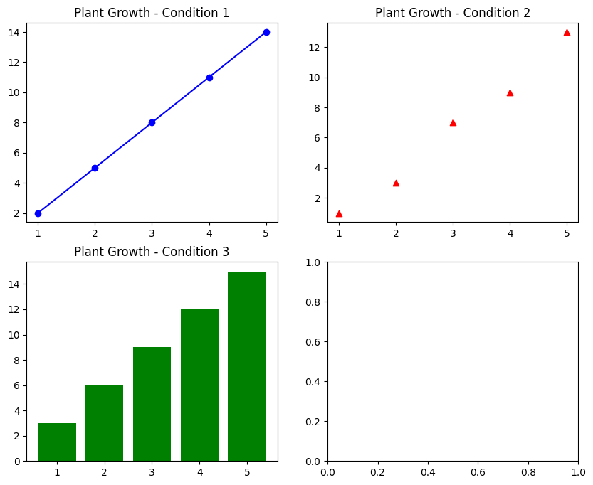
The first subplot (top-left) displays the plant growth under Condition 1 as a line plot (plot() function). It uses blue color with circular markers and sets a title.
# Plotting on the first subplot (top-left) - Line Plot
axs[0, 0].plot(days, condition1, color='blue', marker='o')
axs[0, 0].set_title('Plant Growth - Condition 1')
Output:
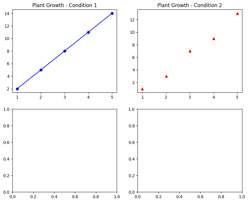
The second subplot (top-right) showcases the plant growth under Condition 2 as a scatter plot (scatter() function). It uses red color with triangle markers and sets a title.
# Plotting on the second subplot (top-right) - Scatter Plot
axs[0, 1].scatter(days, condition2, color='red', marker='^')
axs[0, 1].set_title('Plant Growth - Condition 2')
Output:
The third subplot (bottom-left) visualizes the plant growth under Condition 3 as a bar plot (bar() function) in green color and sets a title.
# Plotting on the third subplot (bottom-left) - Bar Plot
axs[1, 0].bar(days, condition3, color='green')
axs[1, 0].set_title('Plant Growth - Condition 3')
Output:
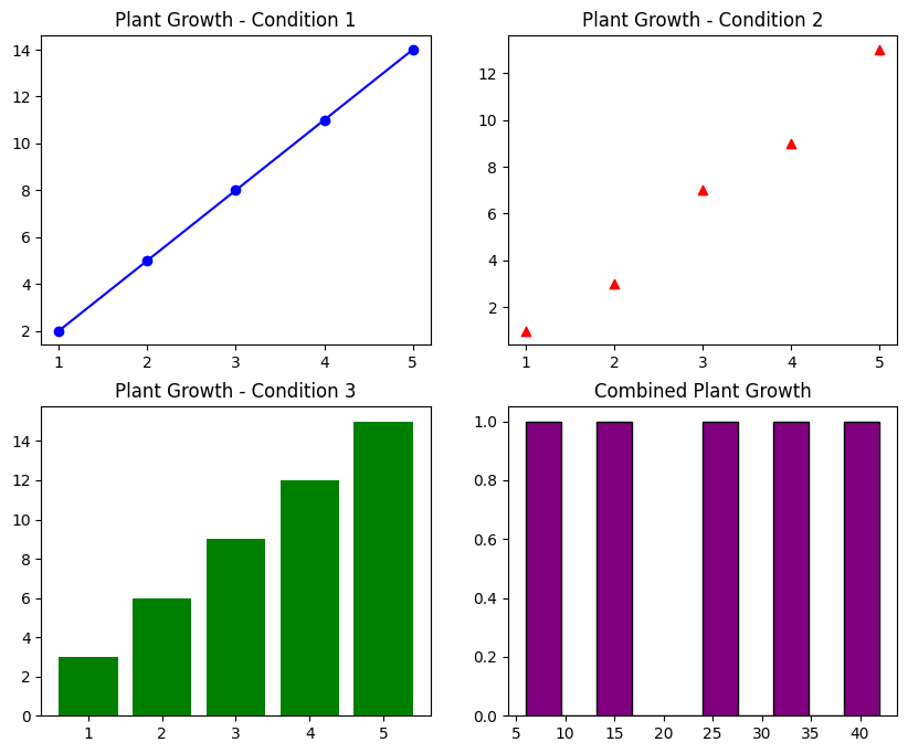
The fourth subplot (bottom-right) shows the combined growth from all conditions as a histogram (hist() function) in purple color. It combines the data from conditions 1, 2, and 3, showcasing their overall distribution and sets a title.
# Plotting on the fourth subplot (bottom-right) - Histogram
axs[1, 1].hist(condition1 + condition2 + condition3, bins=10, color='purple', edgecolor='black')
axs[1, 1].set_title('Combined Plant Growth')
Output:
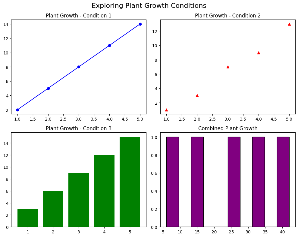
Finally, we add a title to the entire set of subplots and adjust the layout to prevent overlap between them before displaying the plots.
# Adding some overall customization
plt.suptitle('Exploring Plant Growth Conditions', fontsize=16)
plt.tight_layout()

# Display the plots
plt.show()
Output:
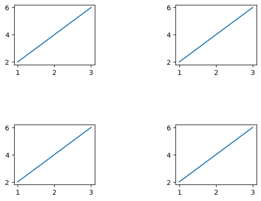
Adjusting Spacing Between Subplots in Matplotlib
You can adjust the spacing between subplots with the help of subplots_adjust() function to improve the layout and appearance of your figures.
The wspace and hspace parameters control the horizontal and vertical spacing between subplots, respectively. Adjust these values to create the ideal balance between your plots.
Example:
# Creating subplots with adjusted spacing
fig, axs = plt.subplots(2, 2)

# Plotting on individual subplots
for i in range(2):
    for j in range(2):
        axs[i, j].plot([1, 2, 3], [2, 4, 6])

# Adjusting spacing between subplots
plt.subplots_adjust(wspace=1, hspace=1)

# Displaying the plot after adjusting spacing
plt.show()
Output:
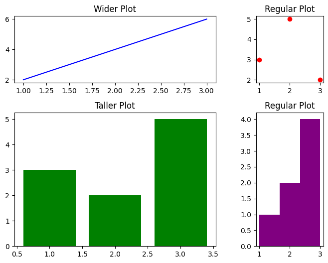
Fine-tuning the Layout of Subplots
Sometimes, the default layout might not be exactly what you’re looking for.
With gridspec_kw, you can specify parameters like width_ratios, and height_ratios. These let you control the relative sizes of subplots.
Example:
# Creating subplots with customized width and height ratios
fig, axs = plt.subplots(2, 2, figsize=(8, 6), gridspec_kw={'width_ratios': [3, 1], 'height_ratios': [1, 2]})

# Plotting on individual subplots
axs[0, 0].plot([1, 2, 3], [2, 4, 6], color='blue')
axs[0, 1].scatter([1, 2, 3], [3, 5, 2], color='red')
axs[1, 0].bar([1, 2, 3], [3, 2, 5], color='green')
axs[1, 1].hist([1, 2, 2, 3, 3, 3, 3], bins=3, color='purple')

# Customizing titles for each subplot
axs[0, 0].set_title('Wider Plot', fontsize=12)
axs[0, 1].set_title('Regular Plot', fontsize=12)
axs[1, 0].set_title('Taller Plot', fontsize=12)
axs[1, 1].set_title('Regular Plot', fontsize=12)

# Adding space between subplots
plt.subplots_adjust(wspace=0.3, hspace=0.3)

plt.show()
In this example, the subplot in the first row and first column is three times wider than the subplot in the second column, while the subplot in the second row and first column is twice as tall as the subplot in the first row. This customization helps emphasize specific plots based on their importance or content.
Output:
Tips for Effective Use of Subplots
| Best Practices and Tips | Avoiding Common Pitfalls |
|---|---|
| Consistent Axes Scaling: Maintain consistent scales across subplots for accurate comparison. | Overcrowding: Avoid cramming too many subplots; keep it clean and easily digestible. |
| Clear Storytelling: Ensure each subplot contributes to the overall narrative without cluttering the visualization. | Unnecessary Repetition: Don’t repeat similar information across multiple subplots unless it’s crucial for comparison. |
| Sensible Layout: Choose an arrangement that complements your data presentation without overwhelming the viewer. | Poor Labeling: Ensure clear labels and titles for each subplot to prevent confusion. |
Exploring Weather Trends: A Real-Life Example
Let’s check out the weather in different cities like New York, Los Angeles, Chicago, and Miami.

First, we’ll look at stuff like temperatures, rainfall, and wind speed for these cities over a year. By seeing this info visually, we can find out interesting things.
import numpy as np

# Generating sample temperature data for different cities
months = np.arange(1, 13)  # Assuming 12 months

# Sample temperature data for each city (replace with actual data if available)
new_york_temperature = np.random.randint(-10, 35, 12)  # Example for New York
los_angeles_temperature = np.random.randint(5, 40, 12)  # Example for Los Angeles
chicago_temperature = np.random.randint(-5, 30, 12)  # Example for Chicago
miami_temperature = np.random.randint(15, 35, 12)  # Example for Miami
And now with Matplotlib’s subplots, we can see each city’s weather data in one place.
Example:
import numpy as np
import matplotlib.pyplot as plt

# Generating sample temperature data for different cities
months = np.arange(1, 13)  # Assuming 12 months

# Sample temperature data for each city (replace with actual data if available)
new_york_temperature = np.random.randint(-10, 35, 12)  # Example for New York
los_angeles_temperature = np.random.randint(5, 40, 12)  # Example for Los Angeles
chicago_temperature = np.random.randint(-5, 30, 12)  # Example for Chicago
miami_temperature = np.random.randint(15, 35, 12)  # Example for Miami

# Your Weather Map Adventure with Subplots
fig, axs = plt.subplots(2, 2, figsize=(10, 8))

# Plotting temperature trends for each city
axs[0, 0].plot(new_york_temperature, label='New York', color='red')
axs[0, 1].plot(los_angeles_temperature, label='Los Angeles', color='blue')
axs[1, 0].plot(chicago_temperature, label='Chicago', color='green')
axs[1, 1].plot(miami_temperature, label='Miami', color='orange')

# Adding titles and labels
axs[0, 0].set_title('New York Temperature')
axs[0, 1].set_title('Los Angeles Temperature')
axs[1, 0].set_title('Chicago Temperature')
axs[1, 1].set_title('Miami Temperature')

# Labels and legends for each city subplot
for ax in axs.flat:
    ax.set_xlabel('Months')
    ax.set_ylabel('Temperature (°C)')
    ax.legend()

plt.tight_layout()
plt.show()
Output:
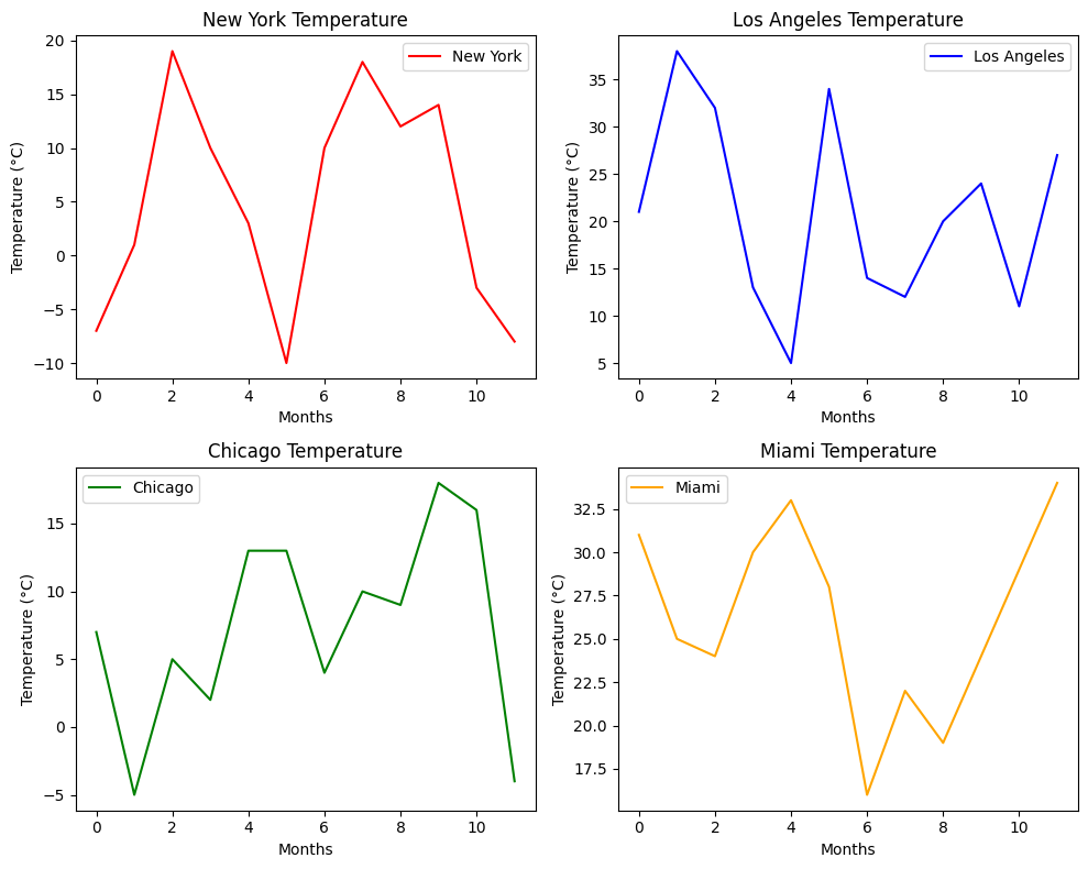
What We Can Learn:
- We can see how temperatures change with the seasons in different cities.
- We’ll spot when it’s hot or cold in each city during the year.
- See how the weather varies from city to city all at once.