Python Random Module Tutorial

The Python random module is a built-in library that allows you to create random numbers and random choices. It’s useful for tasks where you need unpredictability, such as in games, simulations, and data sampling.

This module generates pseudo-random numbers, which means the numbers are generated using algorithms that mimic randomness but are deterministic. This is usually sufficient for most applications but may not be suitable for cryptographic purposes.

The random module is very versatile and can be used in many different scenarios:

• Simulations and Modeling: Creating random events to mimic real-life processes.
• Games and Entertainment: Generating random game elements like dice rolls, shuffled decks of cards, or random enemy movements.
• Data Sampling: Selecting random samples from large datasets for analysis or testing.
• Security: Generating random passwords or keys (although for high-security needs, the secrets module is recommended instead).

Here’s what we will learn in this tutorial.

Getting Started with the Random Module

To use the random module, you first need to import it into your Python program:

import random

Now, let’s learn about the starting functions of the random module.

Generating random numbers using random()

The random.random() function generates a random floating-point number between 0.0 and 1.0, where 0.0 is inclusive and 1.0 is exclusive. This means the result could be any number from 0.0 up to, but not including, 1.0.

Example:

import random

random_number = random.random()
print("Random Number:", random_number)

Output:

Random Number: 0.31941461845381713

Generating random floating-point numbers

If you need a random floating-point number within a specific range, you can use random.uniform(a, b). This function will give you a random float between the values a and b, both inclusive.

Example:

import random

random_float = random.uniform(1.0, 10.0)
print("Random Floating-Point Number:", random_float)

Here, random_float will be a random number like 4.237 or 9.482, and it will be between 1.0 and 10.0.

Output:

Random Floating-Point Number: 5.154605159137677

Generating Random Integers

When working with random numbers in Python, you often need to generate random integers. The random module in Python provides two useful functions for this purpose: randint(a, b) and randrange(start, stop, step).

Using randint(a, b)

The randint(a, b) function generates a random integer between two specified values, a and b. Both a and b are inclusive, meaning the result can be a, b, or any integer in between.

Example:

import random

random_integer = random.randint(1, 10)
print("Random Integer:", random_integer)

When you run this code, you might get any integer between 1 and 10, such as 3, 7, or 10.

Output:

Random Integer: 3

Using randrange(start, stop, step)

The randrange(start, stop, step) function generates a random number from a range that starts at start, ends before stop, and increments by step. This gives you more control over the range and the numbers you get. You can use this function to get a random even number or odd number.

Example:

import random

random_custom = random.randrange(10, 21, 2)
print("Random Custom Integer:", random_custom)

Output:

Random Custom Integer: 16

Generating Random Sequences

The randrange() function is also handy for generating random sequences which can be used for many tasks, like generating random data for simulations or games. You can use the list comprehension with randrange() to create a list of random integers.

Example:

import random

random_sequence = [random.randrange(1, 11) for _ in range(5)]
print("Random Sequence:", random_sequence)

Output:

Random Sequence: [10, 10, 8, 8, 6]

Generating random sequences of even or odd numbers

To generate a sequence of random even numbers, you can specify a step value in randrange(). The step value defines the difference between each number in the range.

Similarly, to generate a sequence of random odd numbers, you can adjust the starting point and step value.

Example:

import random

random_even_sequence = [random.randrange(2, 21, 2) for _ in range(5)]
print("Random Even Sequence:", random_even_sequence)

random_odd_sequence = [random.randrange(1, 20, 2) for _ in range(5)]
print("Random Odd Sequence:", random_odd_sequence)

Output:

Random Even Sequence: [16, 16, 6, 8, 20]
Random Odd Sequence: [11, 7, 1, 17, 5]

Shuffling a List Randomly With shuffle()

Shuffling a list means rearranging its elements in a random order. This is particularly useful in situations where you need to randomize the order of elements. Python’s random module provides a function called shuffle() that makes this easy.

This function takes a list and rearranges its elements randomly. It modifies the original list in place and does not return a new list.

Example:

A common use case for shuffle() is to shuffle a deck of cards.

import random

my_deck = ["Ace", "King", "Queen", "Jack", "10", "9", "8", "7"]
random.shuffle(my_deck)
print("Shuffled Deck:", my_deck)

When you run this code, your list my_deck will be shuffled into a random order.

Output:

Shuffled Deck: ['Ace', '9', '7', '10', 'Jack', 'King', 'Queen', '8']

Randomly Selecting Multiple Elements Without Repetition With sample()

Sometimes, you need to pick several items from a list without choosing the same item more than once. Python’s random module has a function called sample() that makes this easy. This is useful for things like picking random winners for a contest, selecting random survey participants, or any situation where you need a random sample from a list.

The sample() function lets you select a specified number of elements from a list randomly, ensuring the selected elements are unique and do not repeat.

Here’s the syntax:

random.sample(population, k)

• population : The list you want to sample from.
• k : The number of elements you want to select. It must be less than or equal to the length of the list. If k is greater than the number of elements in the list, sample() will raise a ValueError.

Example:

import random

colors = ["red", "blue", "green", "yellow", "orange", "purple"]
random_colors = random.sample(colors, 3)
print("Random Colors:", random_colors)

In this example, you’ll get a list of 3 unique, randomly selected colors from the colors list.

Output:

Random Colors: ['blue', 'purple', 'red']

Selecting Elements Randomly From a List With choice()

Imagine you have a list of items, and you want to pick one item from the list randomly. The choice() function can help you with that. You give it a list, and it gives you back one random element from that list.

This can be handy in many situations, like choosing a random card, selecting a random question from a quiz, or even deciding what to eat for lunch.

Example:

import random

fruits = ["apple", "banana", "cherry", "date", "elderberry"]
random_fruit = random.choice(fruits)
print("Random Fruit:", random_fruit)

This code will select a random fruit from the list.

Output:

Random Fruit: cherry

Random Choices and Weighted Selection Using choices()

The random module offers a helpful function called choices() that lets you make random selections from a list or sequence. This function is quite flexible; you can either make simple random selections or assign weights to the elements, influencing their chances of being picked.

This function is pretty straightforward. You give it a list or sequence of items, and it returns one or more random selections from that list.

Here’s the syntax:

random.choices(sequence, weights=None, k=1)

• sequence : This is the list or sequence from which you want to make selections.
• weights (optional) : You can assign weights to the elements in the sequence. Higher weights mean higher chances of selection.
• k (optional) : This specifies how many selections you want to make. By default, it’s set to 1.

Example:

import random

options = ["candy", "chips", "fruit", "cookie"]
weights = [0.4, 0.2, 0.2, 0.2]

random_choices = random.choices(options, weights=weights, k=5)
print("Random Choices:", random_choices)

Output:

Random Choices: ['candy', 'chips', 'candy', 'cookie', 'candy']

Here’s one more example that shows you the effect of weights more clearly.

Example:

import random

spinwheel=("5 gold coins", "5 silver coins", "1 diamond")

print(random.choices(spinwheel,[10,10,2],k=5))
print(random.choices(spinwheel,[10,0,10],k=3))
print(random.choices(spinwheel,[0,10,10],k=3))
print(random.choices(spinwheel,[0,10,0],k=3))

Output:

['5 silver coins', '5 silver coins', '5 silver coins', '5 gold coins', '5 silver coins']
['5 gold coins', '1 diamond', '1 diamond']
['1 diamond', '1 diamond', '5 silver coins']
['5 silver coins', '5 silver coins', '5 silver coins']

Seed for Reproducibility

Randomness is often crucial in various applications, such as simulations, statistical sampling, and cryptography. However, sometimes you need to reproduce the same sequence of random numbers for debugging, testing, or ensuring consistent results in data analysis. This is where setting a random seed becomes essential. By fixing the seed value, you ensure that the same sequence of random numbers is generated every time you run the code, regardless of the platform or environment.

In Python, you can set a random seed using the seed() function from the random module.

Example:

import random

# Set a random seed
random.seed(45)

# Generate 5 random numbers
for i in range(5):
    print(random.randint(1, 100))

Output:

35
54
63
33
11

The Normal Distribution

A normal distribution is a way to describe how data points are spread out. It’s often called a bell curve because of its shape: most data points are near the middle (mean), and fewer data points are at the ends. The curve is symmetric around the mean.

Normal distribution is important because many real-world phenomena follow this pattern. Examples include heights, test scores, and measurement errors.

By using the gauss() function of random module, you can generate random numbers that follow a normal distribution.

Here’s the syntax:

random.gauss(mu, sigma)

• mu : The mean of the distribution.
• sigma : The standard deviation, which indicates how spread out the numbers are from the mean.

Example:

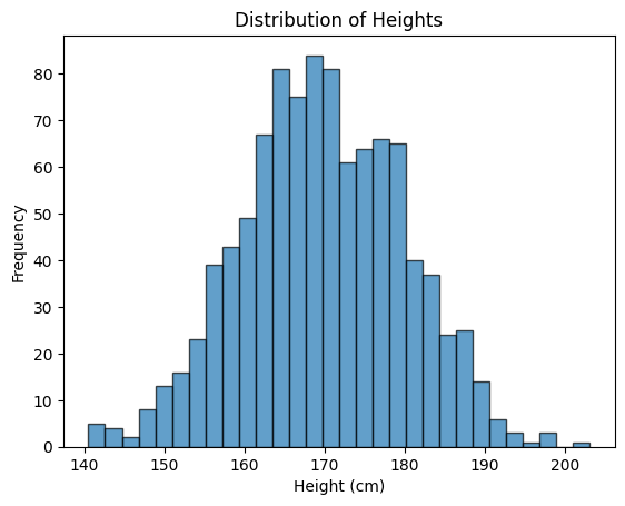
Let’s simulate the heights of people in a group. We’ll use a mean height of 170 cm and a standard deviation of 10 cm. This means most people’s heights are around 170 cm, but some are shorter or taller.

import random
import matplotlib.pyplot as plt

# Set the mean and standard deviation
mean = 170  # Mean height in cm
std_dev = 10  # Standard deviation in cm

# Generate 1000 random heights
heights = [random.gauss(mean, std_dev) for _ in range(1000)]

# Plotting the heights to visualize the distribution
plt.hist(heights, bins=30, edgecolor='black', alpha=0.7)
plt.title("Distribution of Heights")
plt.xlabel("Height (cm)")
plt.ylabel("Frequency")
plt.show()

In this example:

We use a list comprehension to generate 1000 random heights using the random.gauss(mean, std_dev) function.

And for creating the plot we import the matplotlib.pyplot. Then we create a histogram of the heights using plt.hist(), which shows the distribution of heights in the form of a bell curve.

Output:

The Exponential Distribution

An exponential distribution is a way to describe the time between events that happen at a constant average rate.

Exponential distribution is used in many areas such as:

• Queueing Systems: Understanding how long you will wait in line.
• Reliability: Predicting the lifespan of products like electronics. For example, how long a light bulb lasts before it burns out?
• Biology: Modeling the time between events like radioactive decay.

In Python, you can use the expovariate() function from the random module to generate random numbers that follow an exponential distribution. This helps simulate and understand real-world scenarios where the exponential distribution is applicable.

Here’s the syntax:

random.expovariate(lambd)

• lambd : The rate parameter (λ). It represents how often events happen. It’s the inverse of the average waiting time (mean).

Example:

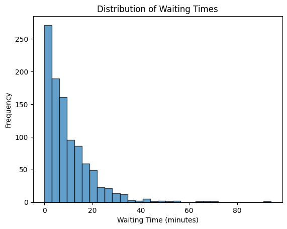
Let’s simulate waiting times for buses that arrive every 10 minutes on average. The rate parameter λ is the inverse of the mean waiting time (1/10 = 0.1).

import random
import matplotlib.pyplot as plt

# Set the rate parameter
rate = 0.1  # Corresponds to an average waiting time of 10 minutes

# Generate 1000 random waiting times
waiting_times = [random.expovariate(rate) for _ in range(1000)]

# Plotting the waiting times to visualize the distribution
plt.hist(waiting_times, bins=30, edgecolor='black', alpha=0.7)
plt.title("Distribution of Waiting Times")
plt.xlabel("Waiting Time (minutes)")
plt.ylabel("Frequency")
plt.show()

When you run the code, you will see a histogram that shows the distribution of waiting times:

• Right-Skewed Shape: The distribution has a long tail to the right, meaning there are fewer long waiting times compared to short ones. This creates a curve that slopes downwards to the right.
• Average Waiting Time: The mean of the distribution is 10 minutes, as expected.

Output:

The Triangular Distribution

A triangular distribution is a way to describe data that has a clear minimum, maximum, and most likely value. It forms a triangle shape when graphed.

Triangular distribution is helpful because it’s simple and easy to understand. It’s often used in situations where:

• Estimating Task Duration: Predicting how long a task might take when you have some idea but not exact data.
• Risk Analysis: Assessing possible outcomes when you don’t have precise information.
• Supply Chain Management: Estimating delivery times when data is limited.

By using the random.triangular() function, you can generate random numbers that follow a triangular distribution. It needs three values: the minimum value, the maximum value, and the most likely value (mode).

Example:

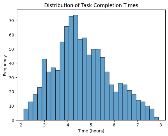
Let’s say you want to estimate the time to complete a task. You think it will take at least 2 hours, at most 8 hours, and most likely 4 hours.

import random
import matplotlib.pyplot as plt

# Set the parameters for the triangular distribution
min_time = 2  # Minimum time in hours
max_time = 8  # Maximum time in hours
mode_time = 4  # Most likely time in hours

# Generate 1000 random completion times
completion_times = [random.triangular(min_time, max_time, mode_time) for _ in range(1000)]

# Plotting the completion times to visualize the distribution
plt.hist(completion_times, bins=30, edgecolor='black', alpha=0.7)
plt.title("Distribution of Task Completion Times")
plt.xlabel("Time (hours)")
plt.ylabel("Frequency")
plt.show()

When you run the code, you will see a histogram that shows how the task completion times are spread out:

• Triangular Shape: The histogram forms a triangle, peaking at the most likely time (4 hours) and sloping down towards the minimum (2 hours) and maximum (8 hours) values.
• Mode: The most likely completion time is where the histogram is highest.

Output:

The Beta Distribution

Beta distribution is a type of probability distribution that is used to describe the probability of different outcomes for a value that ranges between 0 and 1. It is defined by two numbers, called shape parameters: alpha (α) and beta (β). These parameters determine the shape of the distribution.

The Beta distribution is important because it can model different types of data and scenarios. Here are some key uses:

• Bayesian Statistics: Representing prior knowledge about probabilities.
• Project Management: Estimating the time to complete tasks.
• Proportion Data: Analyzing data that represents percentages or proportions, like the success rate of a process.

The betavariate() function helps you to generate random numbers based on a Beta distribution. You just have to specify the alpha (α) and beta (β) parameters.

Example:

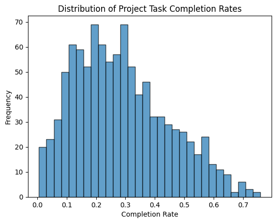
Let’s imagine we want to model the completion rate of a project task. We use α = 2 and β = 5, which means the distribution is skewed towards lower values, suggesting that the task is more likely to be incomplete most of the time.

import random
import matplotlib.pyplot as plt

# Set the alpha and beta parameters
alpha = 2  # Shape parameter α
beta = 5   # Shape parameter β

# Generate 1000 random completion rates
completion_rates = [random.betavariate(alpha, beta) for _ in range(1000)]

# Plotting the completion rates to visualize the distribution
plt.hist(completion_rates, bins=30, edgecolor='black', alpha=0.7)
plt.title("Distribution of Project Task Completion Rates")
plt.xlabel("Completion Rate")
plt.ylabel("Frequency")
plt.show()

When you run the code, you will see a histogram that shows the distribution of project task completion rates:

• Skewed Shape: The histogram will likely show more values close to 0 (indicating lower completion rates).
• Flexible Shape: By changing α and β, you can adjust the shape of the distribution to model different scenarios. For example:
  • If α and β are both greater than 1 and equal, the distribution will be bell-shaped.
  • If α is less than 1 and β is greater than 1, the distribution will be skewed towards 0.
  • If α is greater than 1 and β is less than 1, the distribution will be skewed towards 1.

Output:

The Gamma Distribution

Suppose you’re waiting for a bus, and you want to know how long it will take for the next bus to arrive. The Gamma distribution helps answer questions like these by describing the probability of waiting for a certain amount of time. It’s like having a tool to predict how long you might wait for something to happen.

The Gamma distribution is essential because it helps us understand waiting times and lifetimes in many situations. Here are some use cases:

• Reliability: It helps predict how long things like machines or electronics will last before breaking down.
• Service Waiting Times: It helps estimate how long you might wait for the next customer service representative or the next bus.
• Insurance: It’s used to estimate how long it might take for insurance claims to be made.

With the help of gammavariate() function, you can generate random numbers that follow a Gamma distribution.

To use gammavariate(), we need to give it two parameters: the shape of the distribution and how spread out it is. These are called the shape (k) and scale (θ) parameters.

• k : This controls the shape of the distribution. Higher values mean the peak is sharper.
• theta : This controls how spread out the distribution is. Higher values mean the distribution is more spread out.

Example:

Let’s say we want to know how long it takes for the next customer to arrive at a service point. We’ll use gammavariate() to simulate this scenario.

import random
import matplotlib.pyplot as plt

# Set the shape and scale parameters
k = 2    # Shape parameter
theta = 1  # Scale parameter

# Generate 1000 random waiting times
waiting_times = [random.gammavariate(k, theta) for _ in range(1000)]

# Plotting the waiting times to visualize the distribution
plt.hist(waiting_times, bins=30, edgecolor='black', alpha=0.7)
plt.title("Distribution of Waiting Times")
plt.xlabel("Waiting Time")
plt.ylabel("Frequency")
plt.show()

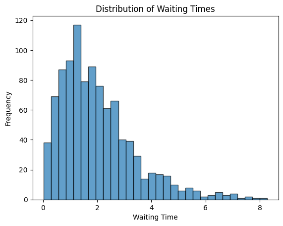
When we plot the waiting times, we see a histogram that shows us how likely it is to wait for different amounts of time:

• Shape: The histogram might look like a curve with a tail on one end. This tail tells us how likely it is to wait for longer times.
• Spread: If the curve is wider, it means we’re likely to wait for a more extended range of times.

Output:

The Log-Normal Distribution

The Log-Normal distribution helps us understand data that are clustered around a central point but have a wide range of possible values. By using the random.lognormvariate() function, we can generate random numbers that follow this distribution.

Here’s why it’s important:

• Financial Markets: Stock prices and financial data often follow a log-normal distribution.
• Biological Sciences: Characteristics like body size or concentrations of substances in biological systems often have a log-normal distribution.
• Engineering: Quantities such as response times or failure times of components in engineering systems often exhibit a log-normal distribution.

To use lognormvariate(), we need to specify two things: the average value (mean) and how spread out the data is (standard deviation) after taking the natural logarithm of the values.

• mu : This is like the middle or average value around which most of the data is clustered.
• sigma : This tells us how spread out the data is. A larger value means the data is more spread out.

Example:

Let’s say we want to simulate the concentrations of a substance in a biological sample. Here’s how we can use lognormvariate():

import random
import matplotlib.pyplot as plt

# Set the mean and standard deviation of the natural logarithm of the distribution
mu = 0.0    # Average concentration
sigma = 0.5  # Spread of the concentrations

# Generate 1000 random concentration values
concentrations = [random.lognormvariate(mu, sigma) for _ in range(1000)]

# Plotting the concentrations to visualize the distribution
plt.hist(concentrations, bins=30, edgecolor='black', alpha=0.7)
plt.title("Distribution of Substance Concentrations")
plt.xlabel("Concentration")
plt.ylabel("Frequency")
plt.show()

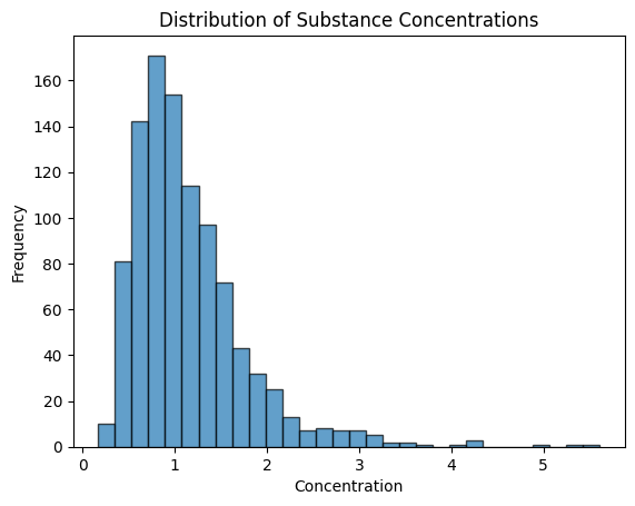
When we plot the concentrations, we see a histogram that shows us how likely it is to observe different concentration values:

• Shape: The histogram might resemble a bell-shaped curve, but it’s skewed towards higher values.
• Spread: The spread of the curve tells us how wide the range of concentration values is.

Output:

The Von Mises Distribution

Now, imagine you’re tracking the direction in which a compass needle points. Most of the time, it might point north, but there could be some variation due to magnetic interference. The Von Mises distribution helps us understand this kind of data, where values are concentrated around a central direction, but there’s some variation around it.

This distribution is commonly seen in many real-life scenarios such as:

• Navigation: It helps model directions in compasses, gyroscopes, or celestial navigation.
• Earth Sciences: It’s used to analyze the orientation of geological structures like fault lines or mineral deposits.
• Signal Processing: It’s useful for modeling phase angles in oscillatory signals like sound waves or electromagnetic waves.

To generate random numbers that follow a Von Mises distribution, you can use the vonmisesvariate() function.

Here’s the syntax:

random.vonmisesvariate(mu, kappa)

• mu : This is the mean direction, where most of the data is clustered around.
• kappa : This parameter controls how spread out the data is. A higher value means less spread.

Example:

Let’s say we want to simulate wind directions at a particular location.

import random
import matplotlib.pyplot as plt
import numpy as np

# Set the mean direction (in radians) and concentration parameter
mu = np.pi/4  # Mean direction (45 degrees)
kappa = 3.0   # Concentration parameter

# Generate 1000 random wind directions
wind_directions = [random.vonmisesvariate(mu, kappa) for _ in range(1000)]

# Convert wind directions from radians to degrees for visualization
wind_directions_degrees = np.degrees(wind_directions)

# Plotting the wind directions to visualize the distribution
plt.hist(wind_directions_degrees, bins=30, edgecolor='black', alpha=0.7)
plt.title("Distribution of Wind Directions")
plt.xlabel("Direction (Degrees)")
plt.ylabel("Frequency")
plt.show()

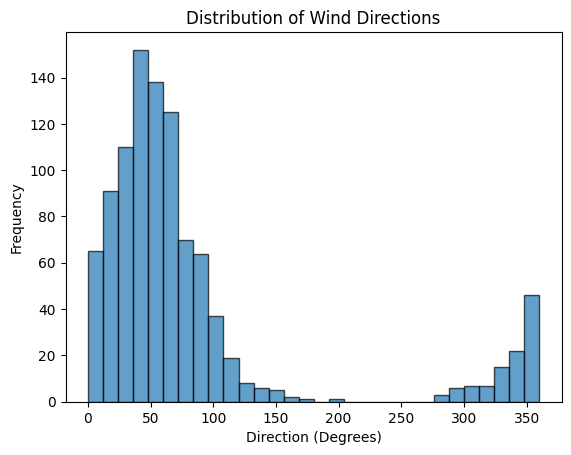
When we look at the histogram, we can see:

• Shape: It’s like a bell-shaped curve, with most wind directions concentrated around the mean direction.
• Spread: The concentration parameter (kappa) controls how spread out the directions are. A higher kappa means less spread.

Output:

The Pareto Distribution

Pareto distribution helps us understand situations where there’s inequality or imbalance. Imagine you’re looking at the distribution of wealth in a society. You might notice that a small percentage of people have most of the wealth, while the majority have much less.

Here are some more use cases of this distribution:

• Natural Phenomena: It describes the distribution of things like the sizes of earthquakes, the wealth of species in ecosystems, or the popularity of websites on the internet.
• Business: It’s used in marketing to understand the distribution of customer lifetime value or the distribution of product sales.

In Python, we can generate random numbers that follow a Pareto distribution using the paretovariate() function. For this function, we only need to specify one parameter, which is the shape of the distribution (alpha). Higher values of alpha mean the distribution decreases more slowly.

Example:

Let’s say we want to simulate the distribution of incomes in a society.

import random
import matplotlib.pyplot as plt

# Set the shape parameter of the Pareto distribution
alpha = 2.5   # Shape parameter

# Generate 1000 random income values
incomes = [random.paretovariate(alpha) for _ in range(1000)]

# Plotting the incomes to visualize the distribution
plt.hist(incomes, bins=30, edgecolor='black', alpha=0.7)
plt.title("Distribution of Incomes")
plt.xlabel("Income")
plt.ylabel("Frequency")
plt.show()

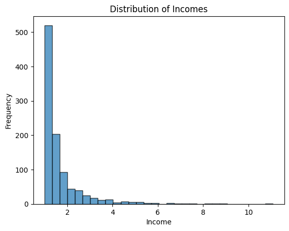
Here, you can see the distribution decreases rapidly at first and then slows down, showing that there are many low incomes and few high-incomes.

Output:

The Weibull Distribution

The Weibull distribution is important because it’s used in many fields to model the failure rates of various products and systems. Imagine you’re studying how long it takes for light bulbs to burn out. Some might fail quickly, while others last much longer. The Weibull distribution helps us describe this kind of data, where the probability of an event happening changes over time.

Here’s why it’s significant:

• Reliability Engineering: It helps predict the lifetimes of components and systems.
• Survival Analysis: It’s used in medical research to study the time until death or failure.
• Extreme Value Theory: It’s employed to analyze the distribution of extreme events, like floods or earthquakes.

The random module provides the weibullvariate() function to generate random numbers that follow a Weibull distribution. To use this, we need to specify two parameters:

• alpha : This parameter controls the shape of the distribution. Higher values mean a more sharply peaked curve.
• beta : This parameter controls the scale of the distribution. Higher values mean a wider spread of data.

Example:

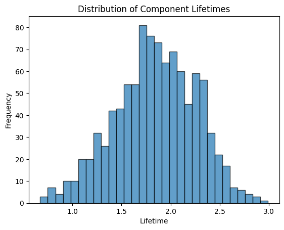
Let’s say we want to simulate the lifetimes of electronic components.

import random
import matplotlib.pyplot as plt

# Set the shape and scale parameters
alpha = 2.0  # Shape parameter
beta = 5.0   # Scale parameter

# Generate 1000 random lifetimes
lifetimes = [random.weibullvariate(alpha, beta) for _ in range(1000)]

# Plotting the lifetimes to visualize the distribution
plt.hist(lifetimes, bins=30, edgecolor='black', alpha=0.7)
plt.title("Distribution of Component Lifetimes")
plt.xlabel("Lifetime")
plt.ylabel("Frequency")
plt.show()

When we look at the histogram, we can see, that it’s like a curve that can be skewed or flattened, depending on the values of alpha and beta. The curve tells us how wide the range of lifetime values is.

Output:

Some Real Life Examples

Randomness plays a crucial role in various real-life applications, making systems unpredictable and secure. Two prominent examples are randomizing elements in game development and generating random passwords for security purposes.

Randomizing Elements in Game Development

In game development, randomness is used to create unpredictable and engaging experiences. This includes generating random events, distributing resources, and creating varied gameplay.

Here’s an example of randomly shuffling a list of items in Python for game development:

Example:

import random

# Create a list of game items
game_items = ["Sword", "Potion", "Shield", "Gold"]

# Shuffle the items randomly
random.shuffle(game_items)
print("Randomly Shuffled Game Items:", game_items)

Output:

Randomly Shuffled Game Items: ['Gold', 'Shield', 'Sword', 'Potion']

Random Password Generation

Creating strong, random passwords is crucial for maintaining security. Randomly generated passwords are less predictable and harder to crack.

Here’s how you can generate a random password with a mix of letters, numbers, and symbols:

Example:

import random
import string

# Define characters for the password
characters = string.ascii_letters + string.digits + string.punctuation

# Generate a random password of length 12
random_password = ''.join(random.choice(characters) for i in range(12))
print("Random Password:", random_password)

Output:

Random Password: *z|@`(1C5.Ja